A Comparison of Least Square, L2-regularization and L1-regularization

Problem Setting

Ordinary Least Square (OLS), L2-regularization and L1-regularization are all techniques of finding solutions in a linear system. However, they serve for different purposes. Recently, L1-regularization gains much attention due to its ability in finding sparse solutions. This post demonstrates this by comparing OLS, L2 and L1 regularization.

Consider the following linear system:

\[Ax = y\]

where \(A \in \reals^{m \times n}\), \(m\) is the number of rows (observations) and \(n\) is the number of columns (variable dimension), \(x\) is the variable coefficients and \(y\) is the response. There are three cases to consider:

1. \(m=n\). This is the common-seen case. If \(A\) is not degenerate, the solution is unique.
2. \(m>n\). This is called over-determined linear system. There is usually no solutions, but an approximation can be easily found by minimizing the residue cost \(\norm{Ax-y}^2_2\) using least square methods, and it has a nice closed-form solution \(x_{ls}=(A^T A)^{-1} A^T y\). In L2-regularization, we add a penalize term to minimize the 2-norm of the coefficients. Thus, the objective becomes: \(\min_x \norm{Ax-y}^2_2 + \alpha \norm{x}_2\) where \(\alpha\) is a weight to decide the importance of the regularization.
3. \(m<n\). This is called under-determined linear system. There is usually no solution or infinite solutions. This is where it get interesting: when we have some prior knowledge in the solution structure, such as sparsity, we can have a ‘metric’ to find a better solution among a whole bunch. The objective is thus: \(\min_x \norm{Ax-y}^2_2 + \alpha \norm{x}_1\) The optimization technique for the above problem is called lasso, and there is an advanced version called elastic net, which combines the L2 and L1 regularization together, hoping to get the advantages of both: L1 regularization finds sparse solution but introduces a large Mean Square Error (MSE) error, while L2 is better at minimizing MSE.

An Example

In the following, we show their performances by solving a simple case.

% regression_ex.m
% Compare Ordinary Least square (no regularization), L2-reguarlized (Ridge),
% L1-regualarized (Lasso) regression in finding the sparse coefficient
% in a underdetermined linear system

rng(0);  % for reproducibility
m = 50;  % num samples
n = 200; % num variables, note that n > m

A = rand(m, n);
x = zeros(n, 1);
nz = 10; % 10 non-zeros variables (sparse)
nz_idx = randperm(n);
x(nz_idx(1:nz)) = 3 * rand(nz, 1);
y = A*x;
y = y + 0.05 * rand(m, 1); % add some noise

% plot original x
subplot(2, 2, 1);
bar(x), axis tight;
title('Original coefficients');

% OLS
x_ols = A \ y;
subplot(2, 2, 2);
bar(x_ols), axis tight;
title('Ordinary Least Square');
y_ols = A * x_ols;

% L2 (Ridge)
x_l2 = ridge(y, A, 1e-5, 0);  % last parameter = 00 to generate intercept term
b_l2 = x_l2(1);
x_l2 = x_l2(2:end);
subplot(2, 2, 3);
bar(x_l2), axis tight;
title('L2 Regularization');
y_l2 = A * x_l2 + b_l2;

% L1 (Lasso)
[x_l1, fitinfo] = lasso(A, y, 'Lambda', 0.1);
b_l1 = fitinfo.Intercept(1);
y_l1 = A * x_l1 + b_l1;
subplot(2, 2, 4);
bar(x_l1), axis tight;
title('L1 Regularization');

% L1 (Elastic Net)
[x_en, fitinfo_en] = lasso(A, y, 'Lambda', 0.1, 'Alpha', 0.7);
b_en = fitinfo_en.Intercept(1);
y_en = A * x_en + b_en;

MSE_y = [mse(y_ols-y), mse(y_l2-y), mse(y_l1-y), mse(y_en-y)];
disp('Mean square error: ')
fprintf('%g    ', MSE_y); fprintf('\n\n');

% Plot the recovered coefficients
figure, hold on
plot(x_l1, 'b');
plot(x_en, 'r');
plot(x, 'g--');
legend('Lasso Coef', 'Elastic Net coef', 'Original Coef');

Output:

Mean square error:
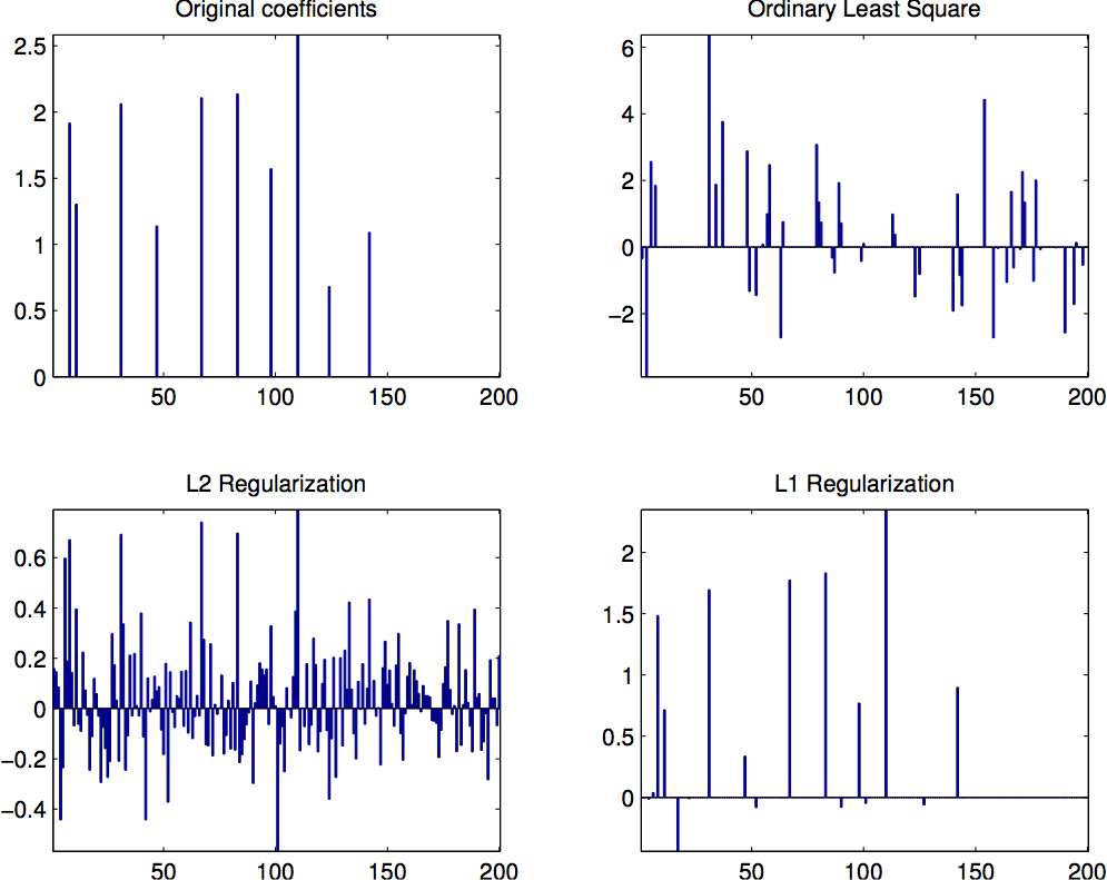
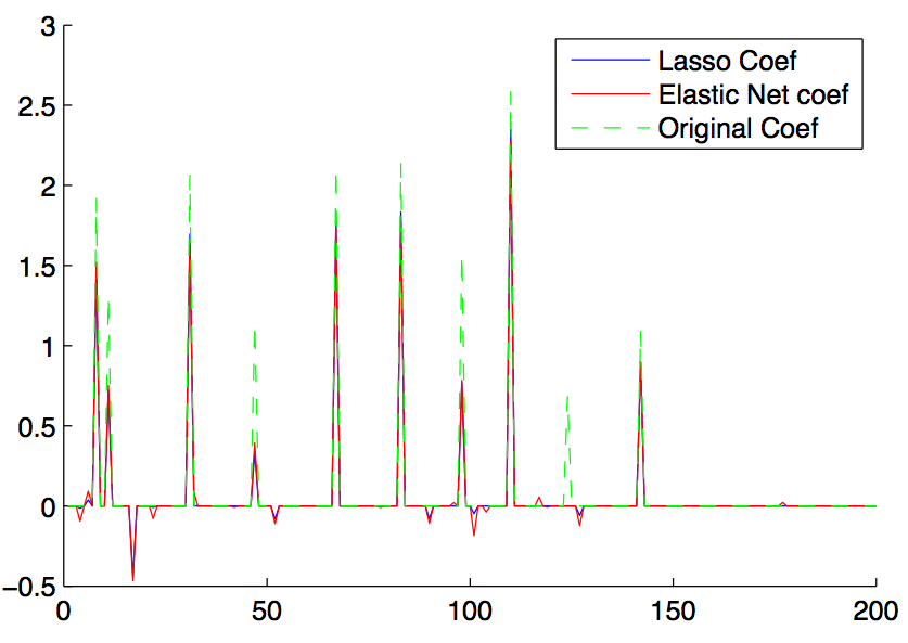
1.81793e-29    7.93494e-15    0.0975002    0.0641214

The above code snippets generates an under-determined matrix \(A\), and a sparse coefficients which has 200 variables but only 10 of them are non-zeros. Noises are added to the responses. We then run the proposed three methods to try to recover the coefficients. It then generates two plots:

1. The first plot is as shown in the top. As we can see, OLS does a very bad job, though the MSE is minimized to zero. L2-regularization do find some of the sparks, but there are also lots of non-zeros introduced. Finally, L1-regularization finds most of the non-zeros correctly and resembles the original coefficients most.
2. The second plot shows how similar the recovered coefficients by lasso and elastic nets resemble the original coefficients. As we can see, both of them can recover most parts, while elastic nets contain some small ‘noise’. However, elastic net yields a slightly better MSE than lasso.

Probing Further

Scikit has some excellent examples on regualarization (1, 2). Quora has an excellent discussion on L2 vs L1 regualarization. I found the top three answers very useful in understanding deeper, especially from the Bayesian regularization paradigm perspective by thinking the regularization as MAP (Maximum A Posteriori) that adds a Laplacian (L1) or Gaussian (L2) prior to the original objective.