Sparse Signal Reconstruction via L1-minimization

This is a follow-up of the previous post on applications of L1 minimization.

As we know, any signal can be decomposed into a linear combination of basis, and the most famous one is Fourier Transform. For simplicity, let’s assume that we have a signal that is a superposition of some sinusoids. For example, the following:

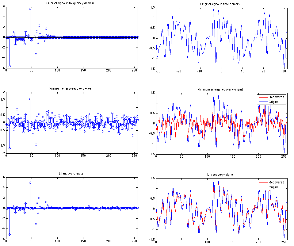
.5*sin(3*x).*cos(.1*x)+sin(1.3*x).*sin(x)-.7*sin(.5*x).*cos(2.3*x).*cos(x);

With discrete consine transform (DCT), we can easily find the coefficients of corresponding sinusoid components. The above example’s coefficients (in frequency domain) and signal in time domain are shown in the post figure.

Now, let’s assume we do not know the signal and want to reconstruct it by sampling. Theorectically, the number of samples required is at least two times the signal frequency, according to the famous Nyquist–Shannon sampling theorem.

However, this assume zero-knowledge about the signal. If we know some structure of the signal, e.g., the DCT coefficients are sparse in our case, we can further reduce the number of samples required. ¹

The following code snippet demonstrates how this works. We generate the original signal in time domain and then perform a DCT to obtain the coefficients.

% sparse signal recovery using L1

rng(0);
N = 256; R = 3; C = 2;

% some superposition of sinoisoids, feel free to change and experiment
f = @(x) .5*sin(3*x).*cos(.1*x)+sin(1.3*x).*sin(x)-.7*sin(.5*x).*cos(2.3*x).*cos(x);
x = linspace(-10*pi, 10*pi, N);
y = f(x);

subplot(R,C,1);
coef = dct(y)';
stem(coef);
xlim([0 N]); title('Original signal in frequency domain');

subplot(R,C,2);
plot(x,y);
xlim([min(x) max(x)]); title('Original signal in time domain');

Let’s assume that we have a device that can sample from the frequency domain. To do this, we create a random measurement matrix to obtain the samples. We use 80 samples here. Note that we normalize the measurement matrix to have orthonormal basis, i.e., the norm of each row is 1, and the dot product of different row is 0.

% measurement matrix
K=80;
A=randn(K, N);
A=orth(A')';

% observations
b=A*coef;

We first try a least-square approach, which boils down to inverse the matrix and obtain \(\hat{x}=A^{-1} b\). Note that as A is not square, we are using its pseudo-inverse here. Furthermore, as A is othornormal, its transpose is the same as pseudo-inverse.

% min-energy observations
c0 = A'*b; % A' = pinv(A) here since A is a full-rank orthonormal matrix
subplot(R,C,3);
stem(c0);
xlim([0 N]); title('Minimum energy recovery - coef');

subplot(R,C,4);
y0 = idct(c0, N);
plot(1:N, y0,'r', 1:N, y, 'b');
xlim([0 N]); title('Minimum energy recovery - signal');
legend('Recovered', 'Original');

As we can see, there are lots of non-zeros in the coefficients, and the recovered signal is very different from the original signal.

Finally, we use L1-minimization for reconstruction. I used lasso to perform a L1-regualarized minimization. Another package that performs various L1-minimization is l1-magic.

% L1-minimization
[c1, fitinfo] = lasso(A, b, 'Lambda', 0.01);
% If use L1-magic
% addpath /path/to/l1magic/Optimization
% [c1] = l1eq_pd(c0, A, [], b, 1e-4);
subplot(R,C,5);
stem(c1);
xlim([0 N]); title('L1 recovery - coef');

subplot(R,C,6);
y1 = idct(c1, N);
plot(1:N, y1, 'r', 1:N, y, 'b');
xlim([0 N]); title('L1 recovery - signal');
legend('Recovered', 'Original');

The above shows that L1-minimization successfully recovered the original signal. A complete code snippet can be found here.

1. In order to recover f perfectly, we need at least \(B \log (N)\) samples (source). ↩